Nonlinear convergence preserves stimulus information

Gabrielle J. Gutierrez, Fred Rieke*, and Eric Shea-Brown*
*co-senior authors

Update: This work is now published in PNAS.

The layered circuitry of the retina compresses and reformats visual inputs before passing them on to the brain. The optic nerve has the channel capacity of an internet connection from the early 90s, yet the brain somehow receives enough information to reconstruct our high-definition world. The goal of this study was to learn something about the compression algorithm of the retina by modeling aspects of its circuit architecture and neural response properties.

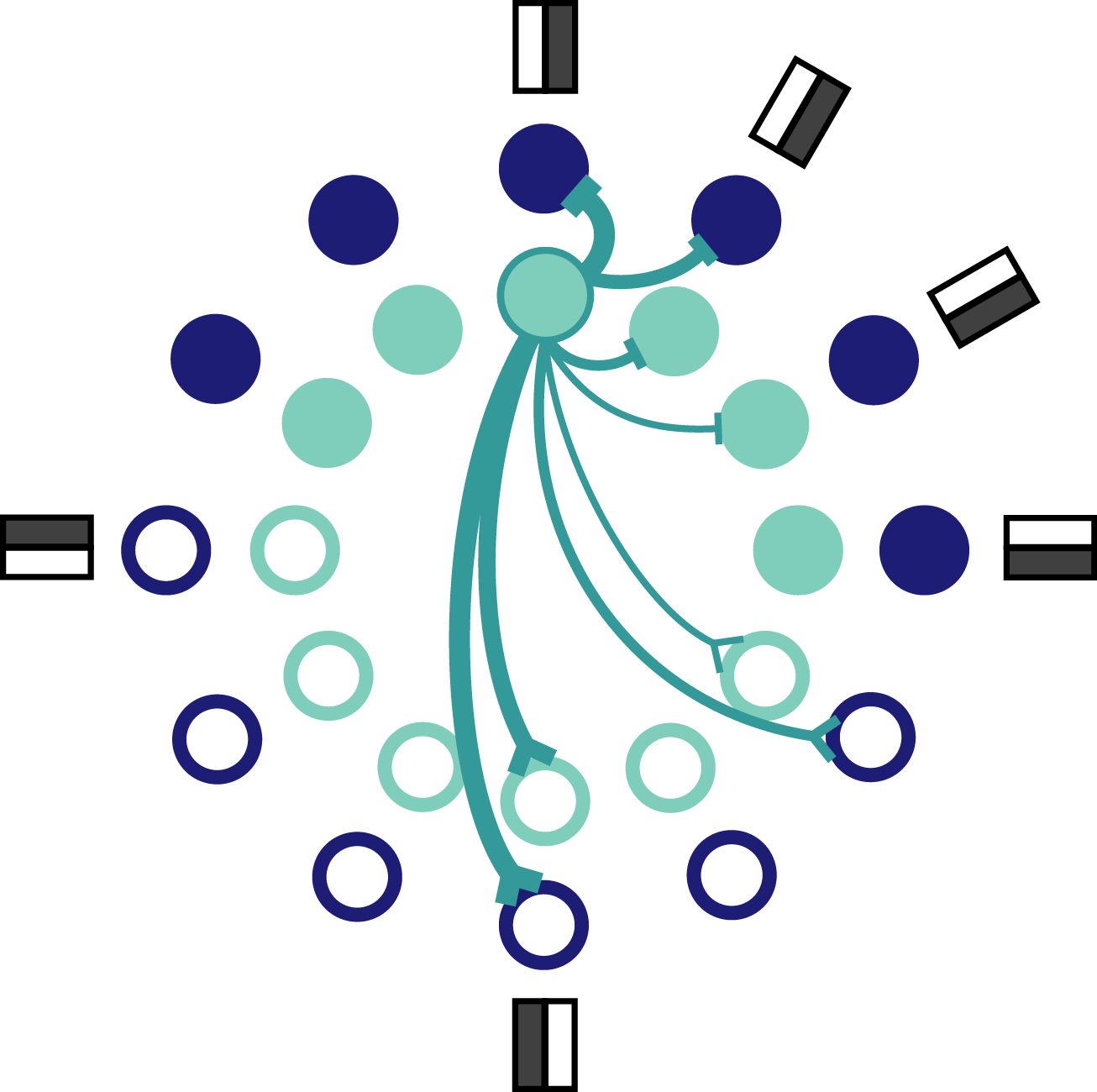
The retina compresses a high-dimensional input into a low-dimensional representation. This is supported by converging and diverging circuit architectures (Fig. 1), along with nonlinear neuron responses. Hundreds of photoreceptors converge to tens of bipolar cells which converge to a single ganglion cell. At the same time, inputs diverge onto many different ganglion cell types that have overlapping receptive fields.

Figure 1: Schematic of retina circuitry illustrating divergence into ON and OFF pathways and convergence within a pathway.

If you look at these circuit components, though, it’s hard to see how they manage to preserve enough information for the brain to work with. For example, converging two inputs can result in ambiguities. In Figure 2, the neural response is simply the sum of the input dimensions. This means that all of the stimuli in the top plot that lie along the orange line are represented by the same response shown by the orange circle in the bottom plot. There’s no telling those stimuli apart, so information is lost by convergence here – down to 12.50 bits in the response from 19.85 bits in the stimulus.

Figure 2: Convergence creates ambiguities, causing information about the stimulus to be lost.

Divergence is another common neural circuit motif. Diverging a stimulus input into two neurons (Fig. 3) expands a 1-dimensional stimulus into a 2-dimensional response but this leads to redundant signals. Here, divergence creates an inefficient neural architecture because it uses two neurons to give you as much information as just one neuron.

Figure 3: Diverging a single inputs into two outputs can produce redundancies.

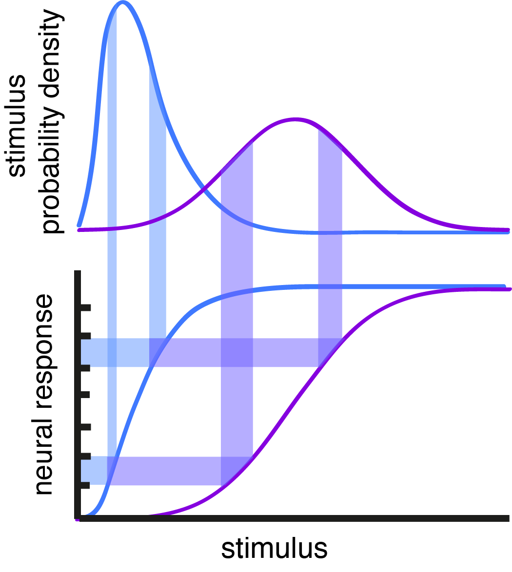
Nonlinear response functions are common in neurons and can make a neuron more efficient at encoding its inputs by spreading its responses around so that information about the stimulus is maximized. Nonlinear response functions can otherwise make a neuron selective to certain stimulus features, but selectivity and efficiency can be in conflict with each other. Figure 4 shows what a rectified linear (ReLU) nonlinearity does to a gaussian stimulus distribution. It compresses the left side of the gaussian so that there is only one response to encode all of the stimuli that fall below the threshold. A lot of information is lost this way. If the stimulus distribution described luminance values in an image, the ReLU would cut out much of the detail from that image.

Figure 4: Nonlinear transformation of a gaussian distributed input with a ReLU can distort the distribution, producing a compressed response where some portion of the stimulus information is discarded.

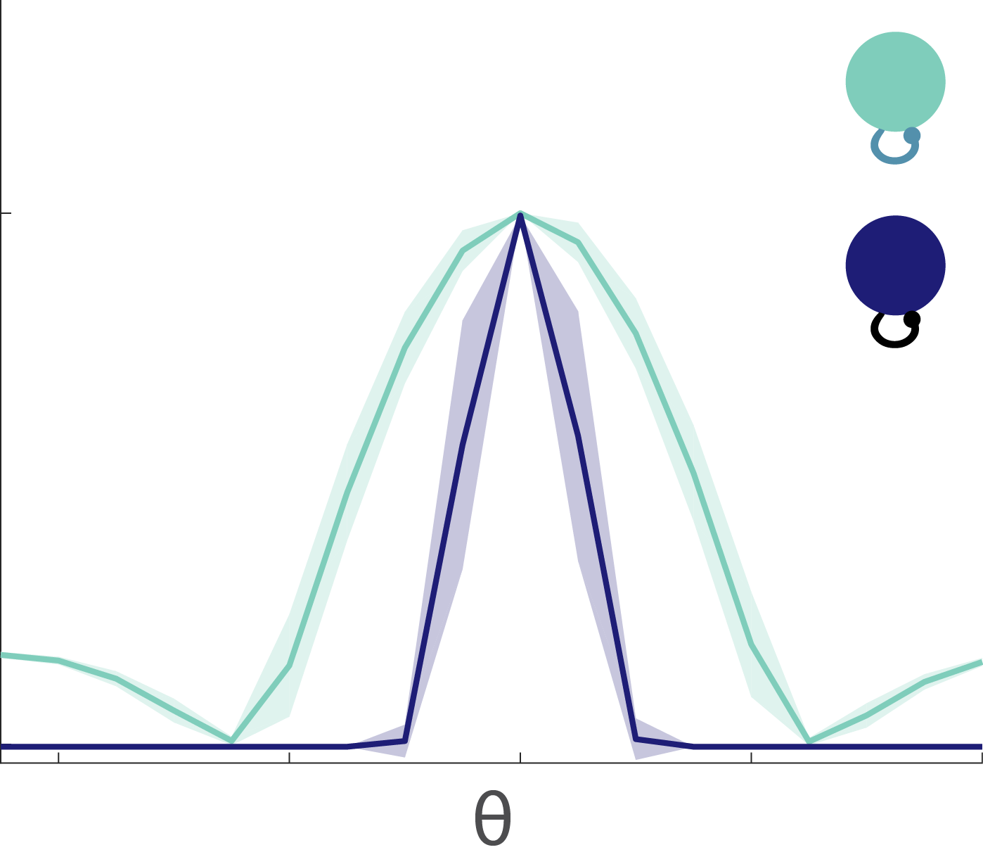
Given that all of these information-problematic elements make up neural circuits, we wondered: how much information can a compressive neural circuit retain when its neurons are nonlinear? We were surprised to find that a convergent, divergent circuit can preserve more information when its subunits are nonlinear than when its subunits are linear (Fig. 5) – even though the individual linear subunits are lossless and the nonlinear subunits are not.

Figure 5: A convergent, divergent circuit with nonlinear subunits (right) preserves more information about the stimulus than a circuit with linear subunits (left).

To explain this, we’ll start out with a reduced version of the circuit. It has only 2 converging subunits and no divergence. Figure 6 shows how a 2-dimensional stimulus is encoded by each layer of the two circuits being compared. The dark purple band represents stimuli whose two inputs sum to the same value. These stimuli are represented by the same output response in the linear subunits circuit as demonstrated by the dark purple that fills a single histogram bin (left, 3rd and 4th rows). Those same stimuli are represented in a more distributed way for the nonlinear subunits circuit (right, 3rd and 4th rows) – meaning that they are represented more distinctly in the output response.

Figure 6: The encoding of the stimulus space at each circuit layer when the subunits are linear (left) and nonlinear (right).

With two subunits, the nonlinear subunits circuit retains more information than the linear subunits circuit, but what happens when there are more than two subunits? The more subunits you compress together, the more difficult it should be to distinguish between different stimuli. Indeed, this is true, but we wondered if the nonlinear subunits circuit would continue to have an advantage over the linear subunits circuit as more subunits are converged. Figure 7 shows that it does. With more subunits, the output response distribution becomes more gaussian, spreading responses out and shifting them towards more positive values (Fig. 7B). The more nonlinear subunits that are converged, the more the nonlinear subunits circuit gains an advantage, up to a saturation point (Fig. 7C). In essence, the convergence of increasing numbers of nonlinear subunits allows the circuit to escape from the compression imposed by the thresholds of the individual nonlinearities themselves.

Figure 7: (A) The output distribution for the linear subunits circuit does not change with more subunits. (B) The output distribution for the nonlinear subunits circuit shifts away from zero and becomes more gaussian. (C) The information entropy for the nonlinear subunits circuit increases with more subunits [subunits undergo an identical normalization regardless of their linearity or nonlinearity].

It would seem that this explains it all; however, there is something subtle to consider. In Figure 5, the circuits had two complementary, diverging pathways – an ON and an OFF pathway. You might have expected the divergence to redeem the linear subunits circuit since the OFF pathway can encode all the stimulus information that the ON pathway discarded. So why is the nonlinear subunits circuit still better? The explanation is in Figure 8 which tracks a distribution of 2-dimensional stimuli through circuits with 2 diverging pathways (ON and OFF) and two subunits in each pathway.

The points are all color-coded by the stimulus quadrant they originated from. The linear subunits don’t meaningfully transform the stimuli (Fig. 8A), although the OFF subunit space is rotated because the OFF subunits put a minus sign on the inputs. When the linear subunits are converged within their respective pathways, the ON and OFF responses compress everything onto a diagonal line because they are perfectly anti-correlated (Fig. 8B). When the output nonlinearities are applied, this linear manifold gets folded into an L-shape (Fig. 8C). Notice how the information entropy for the output response of the linear subunits circuit with diverging pathways is higher than it was with just a single pathway (Fig. 7C, black) – but it has only gone up enough to match the information entropy of a single pathway response without any nonlinearities in either the subunits or the output (Fig. 7C, grey dashed). In other words, the OFF pathway in the linear subunits circuit with output nonlinearities (Fig. 8C) is indeed rescuing the information discarded by the ON pathway, but it cannot do any better than an ON pathway with no nonlinearities anywhere. So how is the nonlinear subunits circuit able to preserve even more information?

Figure 8: Geometrical exploration of the compressive transformations that take place in the linear and nonlinear subunits circuits.

Well, first notice how the nonlinear subunits transform the inputs (Fig. 8D). The nonlinearities actually compress the subunit space, but they do so in complementary ways for the ON and OFF subunits. When these subunits are converged in their respective pathways (Fig. 8E), the output response has some similarities to that for the linear subunits circuit (Fig. 8C). The L-shaped manifold is still there, but the orange and purple points have been projected off of it. These points represent the stimulus inputs with mixed sign. By virtue of having these points leave the manifold and fill out the response space, information entropy is increased. In fact, as more nonlinear subunits are converged in a circuit that also has divergence, the information entropy continues to increase until saturation (Fig. 8F). It even increases beyond that of the fully linear response (shown in Fig. 8B) where there are no nonlinearities anywhere.

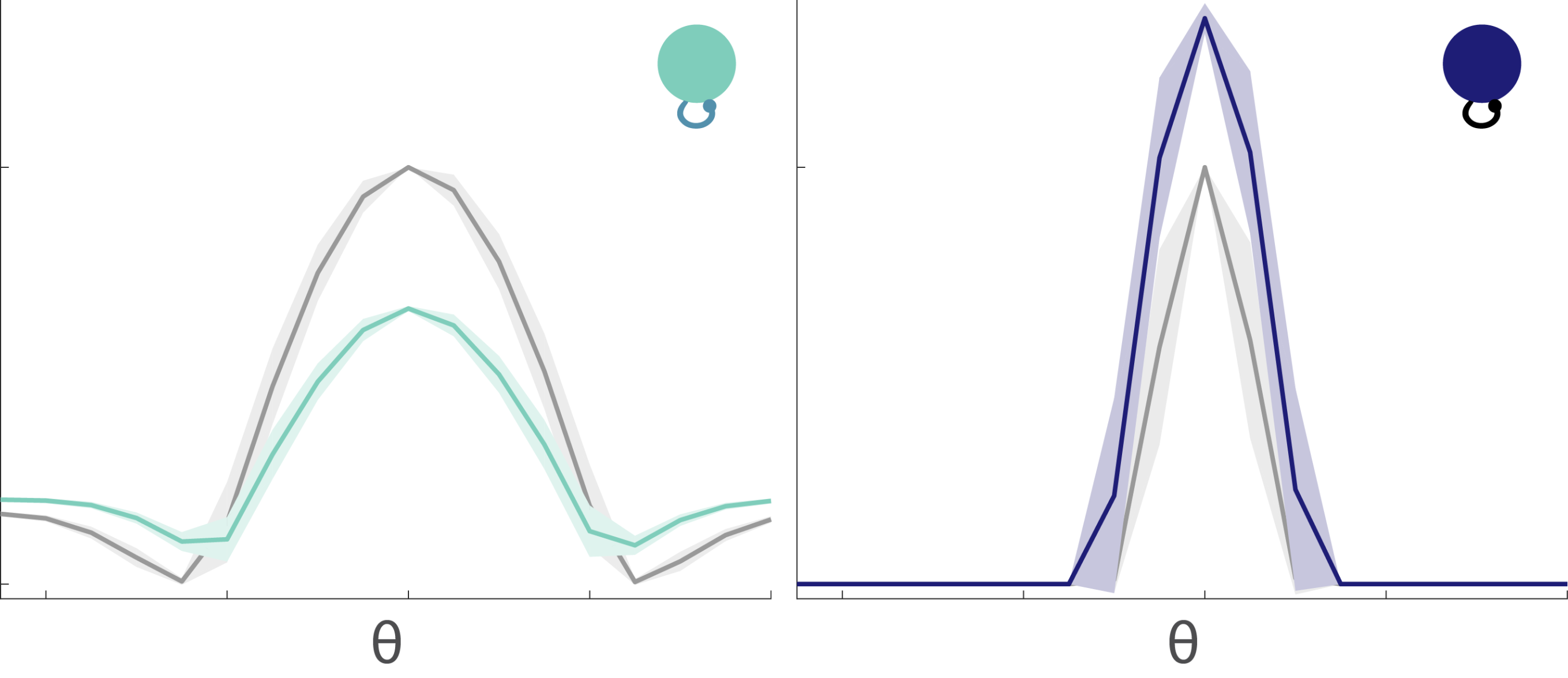
Manifold-schmanifold. Does the nonlinear subunits circuit encode something meaningful for the retina or what? Figure 9 shows that it does! The nonlinear subunits circuit encodes both mean luminance and local contrast whereas the linear subunits circuit is only able to encode the mean luminance of the stimulus. So the convergence of nonlinear subunits not only preserves more quantifiable information, it also preserves more qualitatively useful stimulus information.

Figure 9: (A) The stimulus space is color-coded by bands of of mean luminance. A banded structure is preserved in the output reponse spaces of both the linear and nonlinear subunits circuits. The red square is a reference point. The cyan square has the same mean as the red square, but a different contrast. The red circle has the same contrast as the red square but a different mean. There is no overlap of these shapes in the response space of the nonlinear subunits circuit. (B) The stimulus space is color-coded by contrast levels. The response space of the linear subunits circuit overlaps these levels, providing no distinction between them. The nonlinear subunits circuit preserves separate contrast bands in its response space.

Taken together, what this means for the retina is that the compression algorithm it uses might also be the same one that maximizes information about the stimulus distribution. This is especially noticeable when we focus on the nonlinearity. Nonlinear transformations can induce selectivity, or they can produce an efficient encoding of the stimulus. We’re not used to thinking of them as doing both at the same time though because an efficient code indicates that information about the stimulus is maximized whereas selective coding means that some information about the stimulus will have to be discarded or minimized. My study suggests that selective coding at the single cell level may be leveraged to efficiently encode as much information about the stimulus as possible at the level of the whole circuit.

* a full manuscript of this work is now on bioRxiv – click here

Civilri Whitepaper

My colleague, Adree, and I are interested in finding solutions to the social issues that have emerged from the propagation of information and news via social media. Below is a whitepaper that we wrote together in collaboration with our friend, Malini. It outlines the issues we learned about in our research of the topic.

A race to the top of the frontal cortex.

Applying for a Career Transition K Award from the NIH

Last year, I was awarded a K grant from the NIH. It took two tries and a whole lot of work, but it will set me up for the next few years. I’ll tell you more about what it is, how to apply for one, and why you should apply.

The Career Transition K award funds two more years of postdoc training and the first three years of your first faculty appointment. Commonly it is also called the K99 or K99/R00, but officially, there are other names for it depending on the NIH institution you’re applying to and the particular program. I applied for a K22/R00 through NINDS which was pretty much the same as their K99 but with a focus on minority candidates. I applied for that one because the eligibility requirements allowed me to apply in my fifth year post-grad instead of the cut off of 4 years in the regular K99. My first piece of advice is that you take a good look at all of the K mechanisms at the different NIH institutes and figure out which ones you’re eligible for. Don’t restrict yourself unnecessarily.

NIH Career Development awards

Once you’ve identified a specific K award to apply for at a specific NIH institute, the next thing to do is to contact the program officer for that grant. Let them know that you intend to apply and when. They’ll likely ask to see a draft of your specific aims, so have one ready. They just want a sense of whether you’re eligible and whether your proposed research fits with the institute’s mission. Two reasons why this is important:

Your program officer is your liaison and your advocate. They are there to help you submit your best application and to make sure you’re doing what you can to have the best shot at being funded.
All kinds of hidden factors determine which grant mechanism and institute is the best one for you to apply for. In my case, I thought I’d apply for a K99 at the National Eye Institute (NEI) because my research pertained to computational models of retina circuits. The program officer recommended that I submit to the National Institute for Neurological Disorders and Stroke (NINDS) instead because they had a study section that is more appropriate for evaluating proposals with a computational approach. I never would’ve figured this out on my own.

Once you’ve cleared that, if you haven’t done this before you might think that all you have to do is to write the research proposal and fill out some forms and submit. This isn’t that kind of thing. Your university or institution has significant involvement. You’ll have to contact the administrative office or department that deals with grants. At UW, it’s the office of Sponsored Programs. This has its ups and downs. For one, you’ll have to have your application materials ready weeks in advance of the NIH deadline because your institution has to check it for compliance, approve it, you approve their approval of it, and then they submit it on your behalf. The plus side is that you don’t have to do the whole application by yourself. They fill out most of the copious, tedious forms that go into the grant. This brings me to another point. You won’t have to start from scratch for many of the forms and statements that you’ll submit. You can use past statements from others as a template. For example, statements about lab resources and shared instrumentation, or statements about protocols can easily be modified from ones that likely already exist in your lab or department and that your PI or other trainee had to submit with their grants. Just ask them to share.

So once you’re ready to get going on your application, you should organize yourself. This is a marathon, not a sprint. Make a list or spreadsheet of the application documents and write down who is responsible for completing which ones and your personal deadline for having each part complete. Share it with all who are involved in your application – your PI(s), your grants office, and your department point person if you have one. Use the instruction manual for NIH grant applications (yes, there is one). It lists all the materials that go into these things and provides instructions on what is supposed to be provided in each document. This will give you an idea of whether the documentation is to be provided by you or by an administrative office or your department chair.

Then you can focus on writing a great research proposal and working with your advisor on a training and career development plan. The NIH offers their own guide and tips for writing your application which I found helpful. I also found Anita Devineni’s blog post about her application experience very helpful when I was applying. It was the best guide I had for getting started.

I hope you’ve found this helpful. Don’t be afraid to reach out to others who have done K applications before and ask them to share their completed applications (with all the forms and statements too) and their best advice. Leave comments here or reach out if you have questions for me. Good luck!

How to go about reproducing a conductance-based model and troubleshooting it

Building a model from a publication

All the equations are there, you’ve got figures of model voltage traces that show what the model is supposed to look like, and you’ve got a table of parameters that the authors used to get those figures. It might seem like a breeze to type all that up in Matlab and pop out identical results in reproducing that conductance-based model, but your patience and methodicalness will be rewarded. I recommend starting with the function code that will be called by your ode solver and building in one conductance at a time (see example below).

function dy = myNeuron(t,y)
Vm = y(1); % mV
H = y(2); % gating variable for a conductance
M = y(3);

cm = 1; % nF
g_leak = 0.001; % microS
g_k = 0.2;
g_Na = 0.3;
v_leak = -40; % mV
v_k = -80;
v_Na = 100;

h_inf = 1/(1 + exp((Vm + 15)/6)); % hypothetical steady state gating
m_inf = 0.5*(1 + tanh((Vm - 31)/22));

I_leak = g_leak*(Vm - v_leak); %nA
I_K = g_k*H*(Vm - v_k);
I_Na = g_Na*M*(Vm - v_Na);

dy(1) = (-I_leak - I_Na - I_K)/cm;
dy(2) = (h_inf - H)/tau_h;
dy(3) = (m_inf - M)/tau_m;

This could be your inner function, myNeuron, that is called by the ode solver you choose.

[T,Y] = ode45(@(t,y) myNeuron(t,y),[0 1],y0);

Start with the leak conductance alone – making the most boring, passive neuron ever.

Make sure that no matter what your initial voltage is, the voltage trace that you simulate will relax to the resting voltage you’ve chosen. Does it look like it’s taking too long to get there? Or getting there too quickly? Now is a great time to check your units and the time scale or time step you’re using. If anything about this first step of simulating a passive neuron got weird:

Make sure the units check out. Sometimes authors publish their parameters in terms of conventional units but the units wouldn’t check out on both sides of the equation. For example, without putting a 1e-3 in front of the nA. Below is my little cheatsheet of unit conversions.
Check the implementation of the ode solver you’re using. Make sure the variables haven’t gotten switched, and make sure they’re being assigned to the solver’s channels. Matlab documentation is helpful here: Example of Implementing ODE Solver and Parametrizing Matlab Functions.

unit	conversion
Voltage (Volt)	Current * Time / Capacitance (Ampere * second / Farad)
Current (Ampere)	Charge / Time (Coulomb / second)
Capacitance (Farad)	Charge / Voltage (Coulomb / Volt)
Conductance (Siemen)	1 / Resistance = Current / Voltage (1 / Ohm) = (Ampere / Volt)

giga	1e9
mega	1e6
kilo	1e3
unit	1e0
centi	1e-2
milli	1e-3
micro	1e-6
nano	1e-9
pico	1e-12

If you’ve got a working passive neuron with only a leak conductance, you can start building in the rest of your conductances. I recommend dividing your conductances into “major” and “minor” conductances. The major currents are leak, one main inward, and one main outward current. Work with those first to make sure you get something reasonable that qualitatively resembles a less complex model with only “major” conductances. For example, the Hodgkin-Huxley model only has leak, sodium (Na+), and potassium (K) conductances; or the Morris-Lecar model which has only leak, calcium (Ca), and potassium (K) conductances. Then add in your other currents one at a time and observe that they are changing the model behavior in a way that is expected. For example, including another K conductance should slow down spiking or eliminate it while adding in a Ca conductance should make a more excited response or produce some slow-wave bursting dynamics.

Troubleshooting a complete model

If you’ve gone through the above steps, or if you came to this guide with a complete model that isn’t working. Here are my tips for fixing it.

Stupid things like typos are common. It might not even be your typo but the author’s typo. If possible, check the paper you’re using against another paper that uses the same model. Look for any discrepancies. Generally, the conductance equations should be exactly the same. It’s rare that those change from paper to paper. The parameters would be different from paper to paper (or even within the same paper), but make sure they look reasonable and use comparable units (i.e. it would be weird if one paper used 0.1 picoS for gNa but another paper used 100 mS since the difference is several orders of magnitude and it’s unlikely that both models are functional. Usually one of those is a mistake).
The ode solver may not be right for the model. If you have lots of dynamical variables (>3), the likelihood of stiffness might go up since that can happen with variables that change at very different time scales. One way around this is to choose a very tiny time step while troubleshooting. A tiny time step will eliminate the problem of stiffness for any ode solver you use, so even though it will take much longer to simulate a short run, you can rule out other stuff in the meantime.
Or the simulation time scale is too coarse in general and you’d need to simulate on a finer timescale anyway even if you’ve chosen the best ode solver for your system.
Go through each conductance and do a sign check. Make sure that the conductance produces a current of the correct sign and has qualitatively appropriate dynamics (fast, slow, etc.). Do this with the other currents off. Make sure the current is changing the voltage in a way that seems reasonable/expected (i.e. an inward current should depolarize your voltage).
Look for interdependencies in the conductance equations. If there are any, test those conductances together and make sure one isn’t causing the other to be dysfunctional.

If all else fails, I’ve had success with simply starting from scratch with clean code (no copy/pasting sections of the old code). I know that seems daunting, but you’ll wish you had done it sooner if it solves your problem. I’ve done this before and never ever found the mistake in my original code even though the new code actually worked – so sometimes a small error is really hard to find even when you know it’s in there somewhere.

Crab stomatogastric ganglion dissection guides

When I first started in the Marder Lab as a graduate student, I had the good fortune of being trained in the crab stomatogastric ganglion dissection by a very patient and helpful senior grad student. I also got to watch several other experienced dissectors perform this dissection. This allowed me to come up with my own customized dissection protocol that combined the best aspects of the varied techniques I saw. I wanted to document my dissection protocol in the hopes of helping others who might be trying to learn this dissection, so I made a two-part illustrated guide. This ended up being incorporated into my first official publication in the Journal of Visualized Experiments (Gutierrez and Grashow, 2009).

These guides are still available on the resource page of the Marder lab website, but I’ve made them available here as well.

View this document on Scribd

Dissection part 1 (gross dissection)

Dissection part 2 (fine dissection)

Gutierrez GJ, Grashow RG (2009). Cancer borealis stomatogastric nervous system dissection. J Vis Exp. Mar 23(25). pii: 1207.

“You can’t be what you can’t see”

Since last week, I’ve been running a pilot outreach project in which I Snapchat my day at work. The idea comes from something interesting that I noticed through my more traditional outreach activities, in particular with Girls Who Code. I tend to structure my outreach around the goal of igniting an interest in science, but it quickly becomes clear to me that a deep interest in all things STEM is already burning bright within a lot of the girls who I meet and interact with. In addition to the brilliant questions they ask about my research and the scientific concepts I’ll introduce, they’ll also ask me about what life as a scientist is like. In fact, most of the follow up emails that I receive from these girls are requests to come and visit me at work and to find out more about what it’s like to BE a scientist. Like what do I really do? What kinds of tasks do I carry out? What’s my day to day is like? What is my work environment like? I realized that these questions are about more than a general curiosity about my own life. They’re about whether these girls can see themselves doing what I do – whether they can relate to someone who identifies as both a scientist and a woman of color. So, I’m taking on a small project inspired by a quote from Reshma Saujani, the founder of Girls Who Code – “You can’t be what you can’t see”.

I’m Snapchatting snippets of my work day to give the STEM-curious an inside view of what it’s like to do science. My goal isn’t to teach or explain my research in great detail. That would be impractical given the nature of Snapchat in which posts are really short clips or pictures and expire after 24 hours. My goal is to make my job relatable and less intimidating to anyone interested in science but unsure about whether they can see themselves doing it as a career.

This past week has been fun experimenting with this project, but it’s actually a lot more challenging than I expected. I’m a really private person and I’m not one to pull out my phone and take a random selfie, so I’ve been much more shy than I’d like to be about talking to my phone when my colleagues are around – but I’m trying to be bolder. The other challenge I’m having is with what to show. I do all kinds of things on any given day, but it can be tricky to say something snappy about what I’m working on without much context. That’s where I could use your help. Check out my Snapchat Stories and give me your suggestions for what to present. Also, please share my SnapCode with any young people you know who might be interested in seeing examples of women in science at work. Oh, and one more thing. If you’re doing a job where role models like you are lacking, try doing your own Snapchat thing. We can do it together!

snapcodeBitmoji

E/I balance rescues the decoded representation that is corrupted by adaptation

Gabrielle J. Gutierrez and Sophie Deneve

* Update: this work is now published in the journal eLife.

Spike-frequency adaptation is part of an efficient code, but how do neural networks deal with the adverse effects on the encoded representations they produce? We use a normative framework to resolve this paradox.

Fig. 1: Adaptation shifts response curve. The shift in neural responses maintains a constant response range for an equivalent area under the stimulus PD curve.

The range of firing rates that a neuron can maintain is limited by biophysical constraints and available metabolic resources. Yet, neurons have to represent inputs whose strength varies by orders of magnitude. Early work by Barlow¹ and Laughlin² hypothesized and demonstrated that sensory neurons in early processing centers adapt their response gain as a function of recent input properties (Fig. 1). This work was instrumental in uncovering a principle of neural encoding in which adapting neural responses maximize information transfer. However, the natural follow-up question concerns the decoding of neural responses after they’ve been subject to adaptation. There’s no question that this kind of adaptation has to result in profound changes to the mapping of neural responses to stimuli^3,4 – so how are adapting neural responses interpreted by downstream areas?

By using a normative approach to build a neural network, we show that adapted neural activity can be accurately decoded by a fixed readout unit. This doesn’t require any synaptic plasticity – or re-weighting of the synaptic weights. What it does require, as we’ll show, is a recurrent synaptic structure that promotes E/I balance.

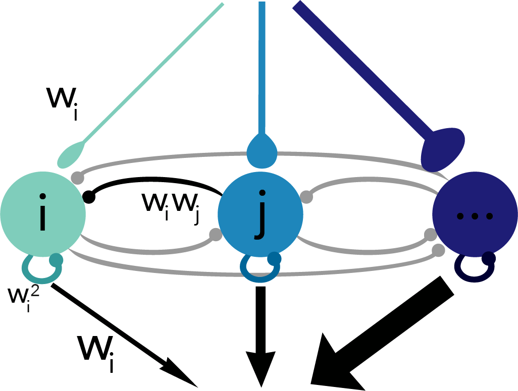
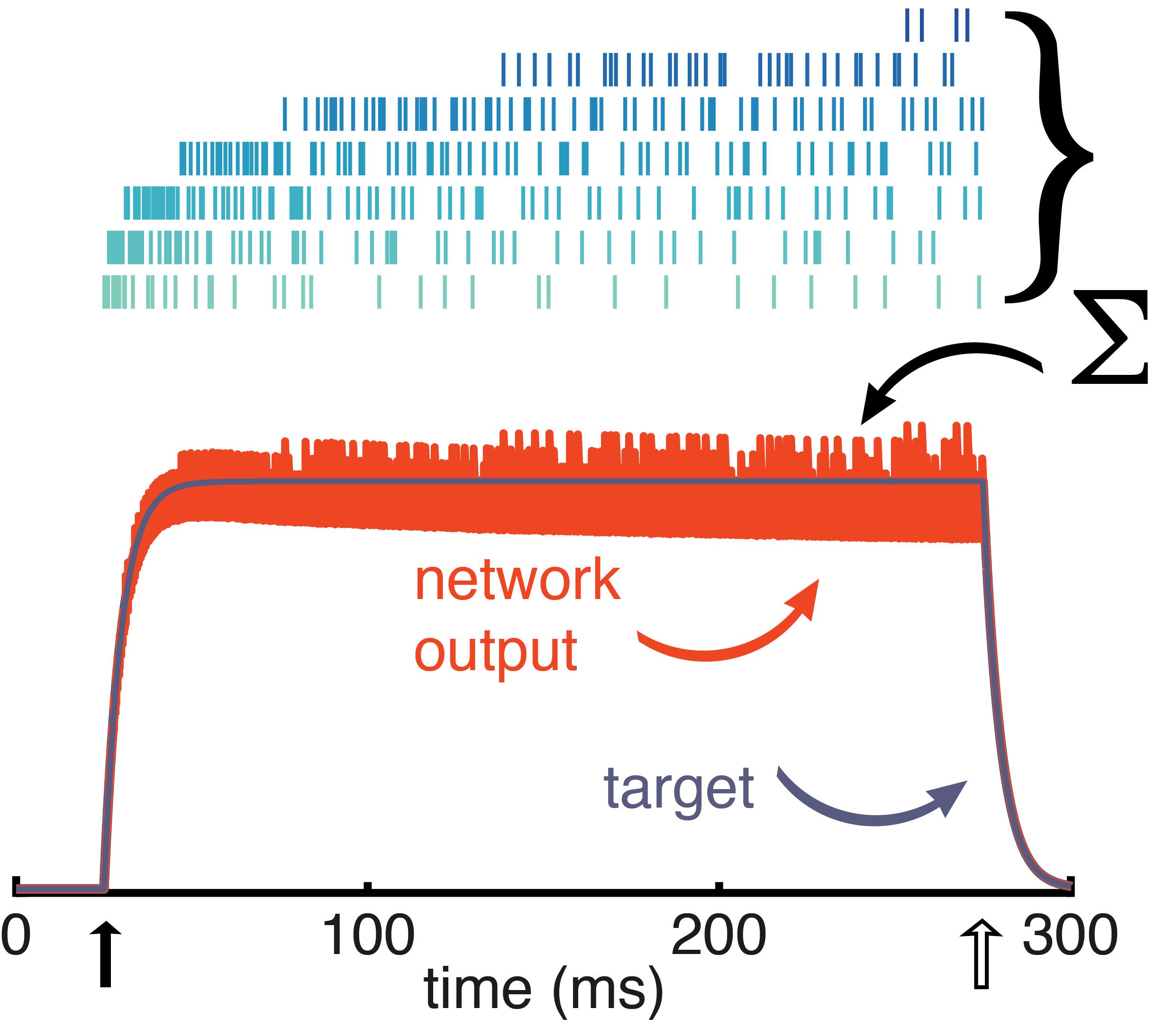
Our approach rests on the premise that nothing is known from the outset about the structure of the network. All we known is the input/output transformation that the network performs. For this study, that I/O function is simply a linear integration of feedforward input the network receives. Given some input, c(t), we expect some output, x(t), such that $\dot{x}(t) = Ax(t) + c(t)$ . The variable, x(t), is called the target signal because it is what we expect the network to produce given the input, but what the network actually puts out is denoted as x̂(t). 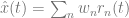We assume that the true network output is a linear sum of the activity of the network units, $\hat{x}(t) = \sum_n w_n r_n(t)$ , where r_i(t) is the activity of neuron i and w_i is its readout weight. It is this actual network output, x̂(t), that will be compared to the target output, x(t).

With these assumptions, we set up an objective function, E, to be minimized. We want to minimize the representation error of the network as well as the overall neural activity. In other words, we derive a network that from the outset has the imperative to be as accurate as possible while also being efficient. The representation error is the squared difference between the decoded estimate that’s read out from the network, x̂, and the output signal we should expect, x, given the input. The metabolic cost is a quadratic penalty on the network firing activity of all n neurons. So the objective looks like this: $E(t) = [x(t) - \hat{x}(t)]^2 + \mu \sum_n r_n(t)^2$

To derive a voltage equation from this objective (see these notes for detailed derivation), we rely on the greedy minimization approach from Boerlin, et al ⁵, which involves setting up an inequality between the objective expression that results when a neuron in the network spikes versus when no spike is fired in the network: E(t|no spike) > E(t|spike). This forces spikes to be informative. A spike may fire only if the objective is minimized by that spike. A spike must make the representation error lower than if a spike were not to have been fired at that time step.

Fig. 2: Spike-frequency adaptation. A history dependent spiking threshold (green) increases and decays with each spike fired (blue) in response to a constant stimulus (pink).

Knowing that the voltage of a spiking neuron needs to cross a threshold before a spike is fired, we let this inequality represent that concept so that after some algebra, the left-hand side expression is taken to be the voltage and the right-hand side is the spiking threshold. In other words, V > threshold is the condition for spiking. Therefore, $V_i = w_i(x - \hat{x}) > \frac{w_i^2 + \mu}{2} + \mu r_i = threshold$ .

Let’s first take a look at the spiking threshold. Notice how it is a function of the neuron activity variable, r(t). This means we’ve derived a dynamic spiking threshold that increases as a function of past spiking activity (Fig. 2). Thus, spike-frequency adaptation fell into our lap from first principles. The dynamic part of this threshold is a direct result of the metabolic cost that was included in the objective function.

Fig. 3: Schematic of derived network.

Taking the derivative of the voltage expression gives us an equation where each term can be interpreted as a current source to the neuron. The resulting network is diagrammed in Figure 3 where you’ll see that the input weight to a given neuron is the same as its readout weight and proportional to the recurrent weights it receives as well as its own self-connection (i.e. autapse). Because our optimization procedure didn’t specify values for these weights – just the relationships between them – the weight parameter, w_i, for any given neuron i is a free parameter. But the value of that parameter has consequences for the adaptation properties of the neuron in question (Fig. 4).

Fig. 4: Adaptation profiles for heterogeneous neurons. The weight parameter determines how excitable a neuron is and its time constant of adaptation.

Neurons with a large weight not only have higher baseline firing thresholds than their small weight counterparts, they have stronger self-inhibition. In contrast, small weight neurons are intrinsically closer to threshold, so they have a higher firing frequency out of the gate, but they burn out quickly because of spike-frequency adaptation. From here on, I’ll refer to the neurons with a small weight as excitable and the large weight neurons as mellow. These heterogeneous adaptation profiles have an important role to play in the network we’ve derived.

Fig. 5: Network response to a stimulus pulse. Neurons fire in response to the stimulus (top, raster) with the most excitable neurons firing first (light green) and the mellower neurons pitching in later (dark blue). Despite time-varying activity in the individual neurons, the network output (orange) tracks the target signal (grey).

To illustrate how this panoply of diverse neurons work together to represent a stimulus, take a look at Figure 5 in which a pulse stimulus has been presented to the network. For the duration of the pulse, the network as a whole does a great job of tracking the stimulus, forming a stable representation over that time. Any single neuron individually does not maintain a stable representation of the stimulus, but the network neurons coordinate as an ensemble. The excitable neurons are the first responders, valiantly taking on the early part of the representation. But they quickly become fatigued. That’s when the mellow neurons kick in to take up the slack. This coordinated effort is all thanks to the recurrent connectivity. When a neuron is firing, it is simultaneously inhibiting other neurons, basically informing other neurons that the stimulus has been accounted for and reported to the readout. But when adaptation starts to fatigue that neuron, it dis-inhibits the other neurons. At some point the amount of input that is going unrepresented outweighs the amount of inhibition coming from the active neuron, causing a mellower neuron to be recruited in carrying the stimulus representation.

Fig. 6: E/I balanced currents reduce error. Left, excitatory and inhibitory currents impinging on an example neuron in response to three different stimulus presentations. The neuron in the top plot belongs to a network with random recurrent connections that are not E/I balanced. In the bottom plot, that neuron is part of an E/I balanced network. Right, the representation error for the unbalanced network (grey) is higher than for the balanced network (black).

This connectivity scheme is inherently E/I balanced, meaning that excitatory currents to an individual neuron are closely tracked to the inhibitory currents entering that same neuron (as shown in the left panel in Fig. 6). When the network takes on a random recurrent structure, even though the currents are somewhat balanced over a long time, they aren’t as tightly balanced as in the recurrent connectivity structure that we derived. The balanced recurrent connectivity scheme is also what’s keeping things accurate (Fig. 6, right plot). In fact, the connectivity structure is entirely derived from the error term in the objective.

Now that we have a model with adaptation and E/I balanced connectivity, we use it to model a network that encodes orientation, such as in area V1 in visual cortex. To do this, we made a neural network with two cell types: mellow and excitable.

Fig. 7: Schematic of orientation coding network. Each orientation is represented by a pair of neurons, one excitable and one mellow neuron. Only a few connections coming from the outlined neuron are shown. Inhibitory connections terminate in a bar and excitatory connections terminate in a prong.

Each neuron has a preferred orientation which is set by the complement of input weights it receives. The preferred orientation of each mellow neuron overlaps with the preference of one other excitable neuron. That means that each orientation is preferred by a pair of network neurons, one excitable and one mellow (Fig. 7). It’s worth pointing out how the derived connectivity interacts with neuron preferences. Specifically, neurons with similar preferences inhibit each other most strongly, whereas neurons with opposing preferences excite each other. This seems counterintuitive – and even contrary to the experimental data – but it reflects the effective encoding strategy at work here. Neurons with similar preferences are competing with each other for the chance to report the stimulus to the readout. If all of the neurons reported at once, the readout would be overwhelmed and unable to decode the stimulus as accurately because the representation would too often reflect the intrinsic properties of the active neurons. On the other hand, neurons with opposite preferences can afford to excite each other because it’s almost like a game of chicken. The active neuron is betting that the opposing neuron isn’t receiving strong input and can therefore feel confident that exciting that neuron won’t be enough to bring it to spike. This set up keeps all neurons relatively close to their baseline spiking thresholds so that any given neuron is ready to be recruited at the drop of a hat.

Fig. 8: Tuning curves. The excitable neurons have broader tuning curves (light green) than the mellow neurons (dark blue).

The tuning curves for the excitable and mellow subpopulations reveal their particular characteristics (Fig. 8). Excitable neurons have a broader tuning curve than their mellow counterparts. Their tuning curves are also higher magnitude than the mellow ones, but both tuning curves were normalized to unity in the figure. These tuning curves represent the early responses of the network neurons to a series of stimulus presentations. By comparing them to the late part of the response to those same stimuli, we can see how the tuning curves change to accommodate the effects of adaptation (Fig. 9). The tuning curve for the late responses in the excitable neurons shows a decrease in the amplitude of the curve near the preferred orientation (left, Fig. 9). This is what most people would expect to see as a result of adaptation. However, the situation for the mellow neurons is counter to those expectations (right, Fig. 9). Their late responses show an increase in activity at the preferred orientation. This is because the excitable neurons are adapted more strongly than the mellow neurons, which means that the mellow neurons have to pitch in to save the representation after the excitable neurons burn out. Thus the mellow neurons tuning curves are facilitated due to adaptation, not suppressed.

Fig. 9: Tuning curves change after adaptation. Tuning curves for early responses as shown in Fig.8 are in grey. After adaptation, the tuning curves are suppressed for the excitable neurons (left, light green), but facilitated for the mellow neurons (right, dark blue).

We showed that E/I balance works hand-in-hand with adaptation to produce a representation that is both efficient and accurate. Sure, we could’ve allowed adaptation to result in a perceptual bias. Our model doesn’t exclude that possibility, but we paid particular attention to the short-term effects of adaptation, and to the subtle changes that adaptation produces in neuron tuning without degrading the network’s ability to accurately encode the stimulus. The bigger picture here is that variability is part of the optimal solution rather than a problem.

Fig. 10: Variability in network neuron responses. The spike rasters from the network are color coded for each stimulus presentation. The stimulus was identical across trials but preceded by a different randomized stimulus sequence. Individual neuron rasters are organized horizontally so that each line represents the spikes from a given neuron.

We illustrate that principle with the overlaid spike rasters in Figure 10 in which the network is presented with the same stimulus on three separate occasions. The only difference between those presentations are the randomized stimulus sequences presented before each one. The history dependence of spike-frequency adaptation produces highly variable neuron responses to the same stimulus over different trials. Despite that variability in the spike timing and firing rate of individual neurons, the network output is very accurate across those three presentations of the stimulus. Adaptation is the catalyst for the redistribution of spikes, while E/I balance is the means by which spiking activity is redistributed in a manner that will preserve the representation. With adaptation enforcing an efficient encoding and E/I balance maintaining an accurate representation, the network can have its cake and eat it too.

Barlow, H. B. Reconstructing the visual image in space and time. Nature 279, 189–190 (1979).
Laughlin, S. A Simple Coding Procedure Enhances a Neurons Information Capacity. Z. Naturforsch., C, Biosci. 36, 910–912 (1981).
Series, P., Stocker, A. A. & Simoncelli, E. P. Is the Homunculus ‘Aware’ of Sensory Adaptation? Neural Comput 21, 3271–3304 (2009).
Solomon, S. G. & Kohn, A. Moving Sensory Adaptation beyond Suppressive Effects in Single Neurons. Current Biology 24, R1012–R1022 (2014).
Boerlin, M., Machens, C. K. & Denève, S. Predictive Coding of Dynamical Variables in Balanced Spiking Networks. PLoS Comput Biol 9, e1003258–16 (2013).

Advice for girls

During one of my visits to a Girls Who Code group, one of the students asked me what advice I have for the next generation of girls. Over the years, I’ve been lucky enough to get some really good advice. So I thought I’d pass it on and also share some things I’ve learned myself.

Make your own mistakes

This was advice given to me by my amazing PhD advisor, Eve Marder. If you don’t make your own mistakes and you let someone else make them for you, you will become “bitter and twisted”. Mistakes are OK, they’re part of being human and part of our learning process. But if you let others dictate your path and allow them to make choices for you, there is nothing to learn. Don’t rob yourself of the personal growth that comes from holding yourself accountable for your choices – even if you’re wrong. Make your own mistakes and make them with courage and conviction!

Value your personal talents

Sometimes you’ll be tempted to assume that what comes easy to you is easy for everyone. Don’t overlook your own talents simply because you have to expend minimal effort to pull them off. It’s especially easy to neglect the things you’re good at when you don’t receive enough encouragement or recognition for them, so when someone complements you for a job well done, don’t write it off as a fluke. You might have a gift that is worth nurturing.

Fake it till you make it

I’ve heard this many times, from many people, and it never stops being good advice. At every stage of your life and career you’ll find yourself doubting your own abilities. It doesn’t help that there will be people who will help to seed that doubt (most without even realizing it). You’re not alone in thinking that you’re not qualified enough, or smart enough for whatever it is you deserve a chance at – it happens to the best. In those times, all you can do is fake it until you convince yourself. If you push on, there will come a point where you realize that you’re drawing on real knowledge and brainpower to “fake” your way through a situation. Confidence can be worn like a coat, and you shouldn’t leave home without it.

Don’t take any opportunity for granted

Sometimes you’ll want to coast through a task because you’re just doing it for your college applications or to check some box somewhere. Other times, you’ll wish you could walk away from an insurmountable challenge or you might be too intimidated to even try in the first place. Yet these are all opportunities to do something awesome, to learn about yourself and the world, and to gain skills or knowledge that you didn’t have before. Don’t take them for granted. You’ll be better off if you make the most out of the experiences and the challenges you take on, so go all the way!

About BiasWatchNeuro

The goal of this site is to track the speaker composition of conferences in neuroscience, particularly with respect to gender representation. The progress of science benefits from diverse voices and ideas. Conference panels that are diverse with respect to gender, race, ethnicity and national origin help advance this goal. Homogenous conference programs are generally not representing their field, missing out on important scientific findings, and are one important factor contributing to the “brain-drain” of talented female and minority scientists from the scientific workforce. As a group, BiasWatchNeuro has formed to encourage conference organizers to make every effort to compose programs that incorporate diverse panels.

Bias is often unconscious and unintended. Indeed, most of us are biased, but with appropriate awareness, many people are now successful at overcoming their biases. The purpose of this site is to provide data and other resources to facilitate that effort, and in particular, to raise awareness of any gender bias in the selection of conference speakers, so that these disparities can be addressed. See “how can I help” for more information.

Send information about conferences, seminar series or other scientific programs to biaswatchneuro@gmail.com

Source: About

Hello world! I’m a girl who codes!

This summer, I volunteered to be a guest speaker at Girls Who Code and it was an amazing experience! Girls Who Code is an organization that teaches high school girls the fundamentals of writing code while they work through some really neat projects. They start from “Scratch” and work their way up to Python – an impressive course load for a summer program.

Programs like these are crucial for getting more women into STEM fields where they’re currently underrepresented. I had the privilege of telling them about my research and about my path to becoming a computational neuroscientist.

I highly recommend these kinds of outreach opportunities to any of my friends and colleagues. It’s definitely worth making time for because just a couple of hours out of your busy schedule can influence the trajectory of someone else’s life. It’s so important for the next generation of girls to see examples of other girls who entered a field they had never seen themselves in. And it’s even more important for girls to know that the women who’ve made it were just as intimidated and unsure when they were girls themselves. Another reason I recommend doing this kind of outreach is because there is something cathartic about reflecting on how far you’ve come from when you were their age. Lighting up another girl’s path is the ultimate reward for all the obstacles and battles with self-doubt you’ve endured in reaching for your own dream STEM career.

P.S. Girls Who Code just started a fundraiser to continue offering this spectacular opportunity to learn to code to more girls. Check it out!

Gabrielle J Gutierrez

Computational Neuroscientist