
Gabrielle J. Gutierrez and Sophie Deneve
* Update: this work is now published in the journal eLife.
Spike-frequency adaptation is part of an efficient code, but how do neural networks deal with the adverse effects on the encoded representations they produce? We use a normative framework to resolve this paradox.

Fig. 1: Adaptation shifts response curve. The shift in neural responses maintains a constant response range for an equivalent area under the stimulus PD curve.
The range of firing rates that a neuron can maintain is limited by biophysical constraints and available metabolic resources. Yet, neurons have to represent inputs whose strength varies by orders of magnitude. Early work by Barlow1 and Laughlin2 hypothesized and demonstrated that sensory neurons in early processing centers adapt their response gain as a function of recent input properties (Fig. 1). This work was instrumental in uncovering a principle of neural encoding in which adapting neural responses maximize information transfer. However, the natural follow-up question concerns the decoding of neural responses after they’ve been subject to adaptation. There’s no question that this kind of adaptation has to result in profound changes to the mapping of neural responses to stimuli3,4 – so how are adapting neural responses interpreted by downstream areas?
By using a normative approach to build a neural network, we show that adapted neural activity can be accurately decoded by a fixed readout unit. This doesn’t require any synaptic plasticity – or re-weighting of the synaptic weights. What it does require, as we’ll show, is a recurrent synaptic structure that promotes E/I balance.
Our approach rests on the premise that nothing is known from the outset about the structure of the network. All we known is the input/output transformation that the network performs. For this study, that I/O function is simply a linear integration of feedforward input the network receives. Given some input, c(t), we expect some output, x(t), such that 
With these assumptions, we set up an objective function, E, to be minimized. We want to minimize the representation error of the network as well as the overall neural activity. In other words, we derive a network that from the outset has the imperative to be as accurate as possible while also being efficient. The representation error is the squared difference between the decoded estimate that’s read out from the network, x̂, and the output signal we should expect, x, given the input. The metabolic cost is a quadratic penalty on the network firing activity of all n neurons. So the objective looks like this:
![E(t) = [x(t) - \hat{x}(t)]^2 + \mu \sum_n r_n(t)^2](https://s0.wp.com/latex.php?latex=E%28t%29+%3D+%5Bx%28t%29+-+%5Chat%7Bx%7D%28t%29%5D%5E2+%2B+%5Cmu+%5Csum_n+r_n%28t%29%5E2&bg=ffffff&fg=656565&s=0&c=20201002)
To derive a voltage equation from this objective (see these notes for detailed derivation), we rely on the greedy minimization approach from Boerlin, et al 5, which involves setting up an inequality between the objective expression that results when a neuron in the network spikes versus when no spike is fired in the network: E(t|no spike) > E(t|spike). This forces spikes to be informative. A spike may fire only if the objective is minimized by that spike. A spike must make the representation error lower than if a spike were not to have been fired at that time step.
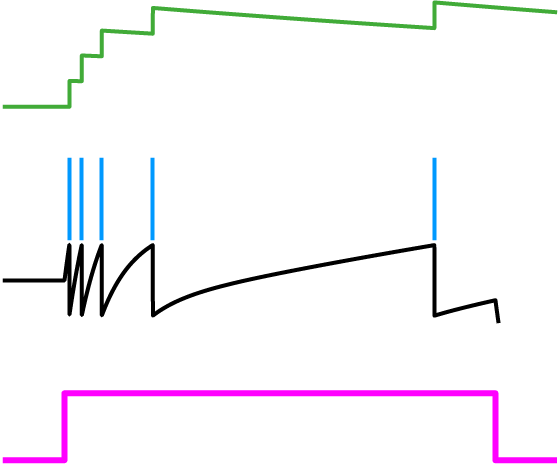
Fig. 2: Spike-frequency adaptation. A history dependent spiking threshold (green) increases and decays with each spike fired (blue) in response to a constant stimulus (pink).
Knowing that the voltage of a spiking neuron needs to cross a threshold before a spike is fired, we let this inequality represent that concept so that after some algebra, the left-hand side expression is taken to be the voltage and the right-hand side is the spiking threshold. In other words, V > threshold is the condition for spiking. Therefore, 
Let’s first take a look at the spiking threshold. Notice how it is a function of the neuron activity variable, r(t). This means we’ve derived a dynamic spiking threshold that increases as a function of past spiking activity (Fig. 2). Thus, spike-frequency adaptation fell into our lap from first principles. The dynamic part of this threshold is a direct result of the metabolic cost that was included in the objective function.

Fig. 3: Schematic of derived network.
Taking the derivative of the voltage expression gives us an equation where each term can be interpreted as a current source to the neuron. The resulting network is diagrammed in Figure 3 where you’ll see that the input weight to a given neuron is the same as its readout weight and proportional to the recurrent weights it receives as well as its own self-connection (i.e. autapse). Because our optimization procedure didn’t specify values for these weights – just the relationships between them – the weight parameter, wi, for any given neuron i is a free parameter. But the value of that parameter has consequences for the adaptation properties of the neuron in question (Fig. 4).
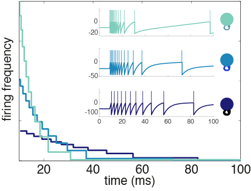
Fig. 4: Adaptation profiles for heterogeneous neurons. The weight parameter determines how excitable a neuron is and its time constant of adaptation.
Neurons with a large weight not only have higher baseline firing thresholds than their small weight counterparts, they have stronger self-inhibition. In contrast, small weight neurons are intrinsically closer to threshold, so they have a higher firing frequency out of the gate, but they burn out quickly because of spike-frequency adaptation. From here on, I’ll refer to the neurons with a small weight as excitable and the large weight neurons as mellow. These heterogeneous adaptation profiles have an important role to play in the network we’ve derived.

Fig. 5: Network response to a stimulus pulse. Neurons fire in response to the stimulus (top, raster) with the most excitable neurons firing first (light green) and the mellower neurons pitching in later (dark blue). Despite time-varying activity in the individual neurons, the network output (orange) tracks the target signal (grey).
To illustrate how this panoply of diverse neurons work together to represent a stimulus, take a look at Figure 5 in which a pulse stimulus has been presented to the network. For the duration of the pulse, the network as a whole does a great job of tracking the stimulus, forming a stable representation over that time. Any single neuron individually does not maintain a stable representation of the stimulus, but the network neurons coordinate as an ensemble. The excitable neurons are the first responders, valiantly taking on the early part of the representation. But they quickly become fatigued. That’s when the mellow neurons kick in to take up the slack. This coordinated effort is all thanks to the recurrent connectivity. When a neuron is firing, it is simultaneously inhibiting other neurons, basically informing other neurons that the stimulus has been accounted for and reported to the readout. But when adaptation starts to fatigue that neuron, it dis-inhibits the other neurons. At some point the amount of input that is going unrepresented outweighs the amount of inhibition coming from the active neuron, causing a mellower neuron to be recruited in carrying the stimulus representation.
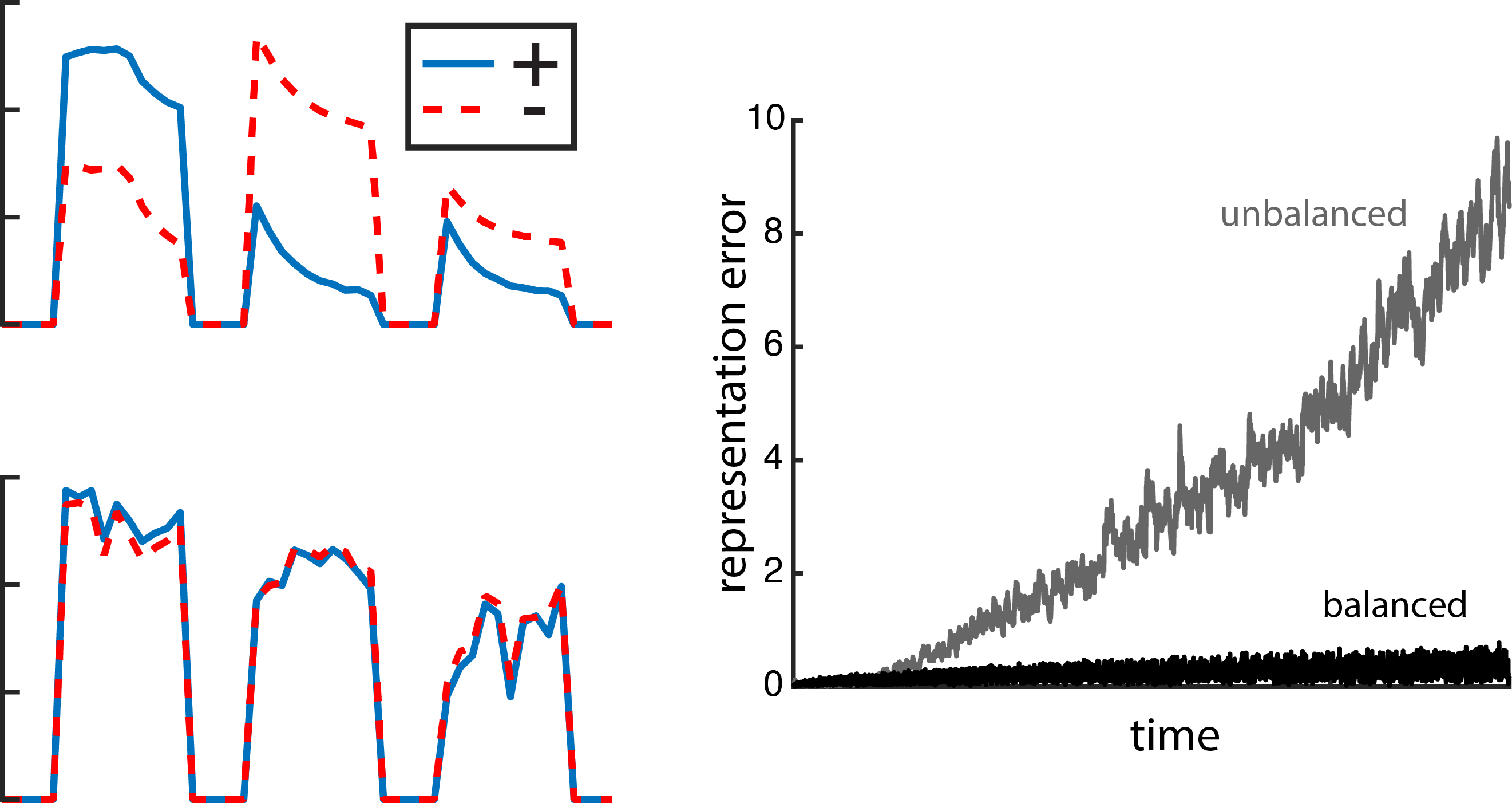
Fig. 6: E/I balanced currents reduce error. Left, excitatory and inhibitory currents impinging on an example neuron in response to three different stimulus presentations. The neuron in the top plot belongs to a network with random recurrent connections that are not E/I balanced. In the bottom plot, that neuron is part of an E/I balanced network. Right, the representation error for the unbalanced network (grey) is higher than for the balanced network (black).
This connectivity scheme is inherently E/I balanced, meaning that excitatory currents to an individual neuron are closely tracked to the inhibitory currents entering that same neuron (as shown in the left panel in Fig. 6). When the network takes on a random recurrent structure, even though the currents are somewhat balanced over a long time, they aren’t as tightly balanced as in the recurrent connectivity structure that we derived. The balanced recurrent connectivity scheme is also what’s keeping things accurate (Fig. 6, right plot). In fact, the connectivity structure is entirely derived from the error term in the objective.
Now that we have a model with adaptation and E/I balanced connectivity, we use it to model a network that encodes orientation, such as in area V1 in visual cortex. To do this, we made a neural network with two cell types: mellow and excitable.
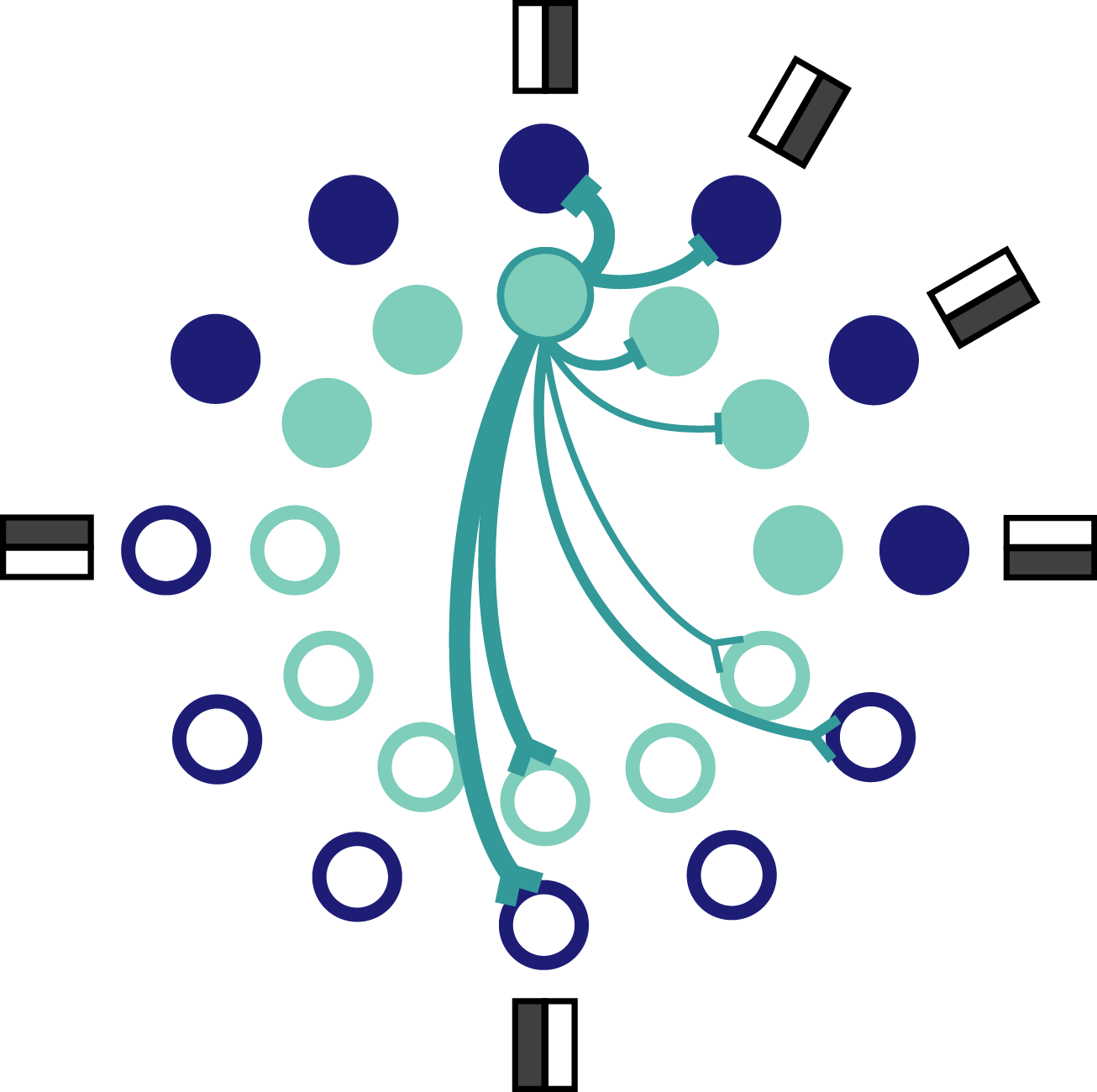
Fig. 7: Schematic of orientation coding network. Each orientation is represented by a pair of neurons, one excitable and one mellow neuron. Only a few connections coming from the outlined neuron are shown. Inhibitory connections terminate in a bar and excitatory connections terminate in a prong.
Each neuron has a preferred orientation which is set by the complement of input weights it receives. The preferred orientation of each mellow neuron overlaps with the preference of one other excitable neuron. That means that each orientation is preferred by a pair of network neurons, one excitable and one mellow (Fig. 7). It’s worth pointing out how the derived connectivity interacts with neuron preferences. Specifically, neurons with similar preferences inhibit each other most strongly, whereas neurons with opposing preferences excite each other. This seems counterintuitive – and even contrary to the experimental data – but it reflects the effective encoding strategy at work here. Neurons with similar preferences are competing with each other for the chance to report the stimulus to the readout. If all of the neurons reported at once, the readout would be overwhelmed and unable to decode the stimulus as accurately because the representation would too often reflect the intrinsic properties of the active neurons. On the other hand, neurons with opposite preferences can afford to excite each other because it’s almost like a game of chicken. The active neuron is betting that the opposing neuron isn’t receiving strong input and can therefore feel confident that exciting that neuron won’t be enough to bring it to spike. This set up keeps all neurons relatively close to their baseline spiking thresholds so that any given neuron is ready to be recruited at the drop of a hat.
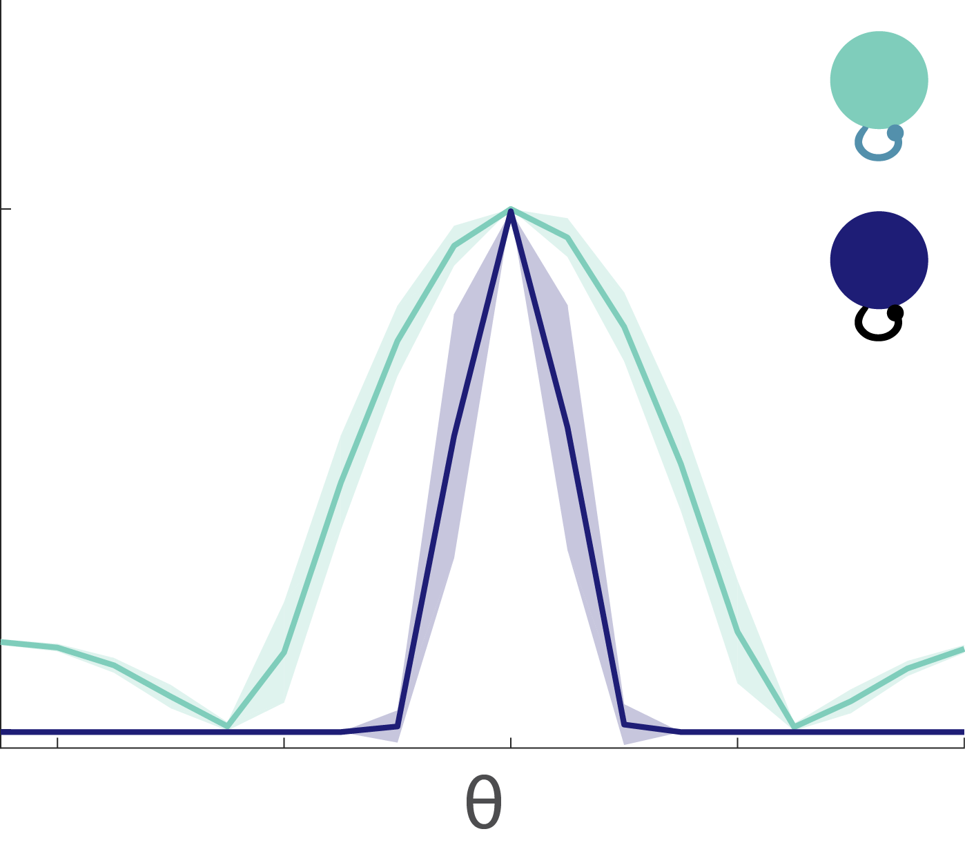
Fig. 8: Tuning curves. The excitable neurons have broader tuning curves (light green) than the mellow neurons (dark blue).
The tuning curves for the excitable and mellow subpopulations reveal their particular characteristics (Fig. 8). Excitable neurons have a broader tuning curve than their mellow counterparts. Their tuning curves are also higher magnitude than the mellow ones, but both tuning curves were normalized to unity in the figure. These tuning curves represent the early responses of the network neurons to a series of stimulus presentations. By comparing them to the late part of the response to those same stimuli, we can see how the tuning curves change to accommodate the effects of adaptation (Fig. 9). The tuning curve for the late responses in the excitable neurons shows a decrease in the amplitude of the curve near the preferred orientation (left, Fig. 9). This is what most people would expect to see as a result of adaptation. However, the situation for the mellow neurons is counter to those expectations (right, Fig. 9). Their late responses show an increase in activity at the preferred orientation. This is because the excitable neurons are adapted more strongly than the mellow neurons, which means that the mellow neurons have to pitch in to save the representation after the excitable neurons burn out. Thus the mellow neurons tuning curves are facilitated due to adaptation, not suppressed.
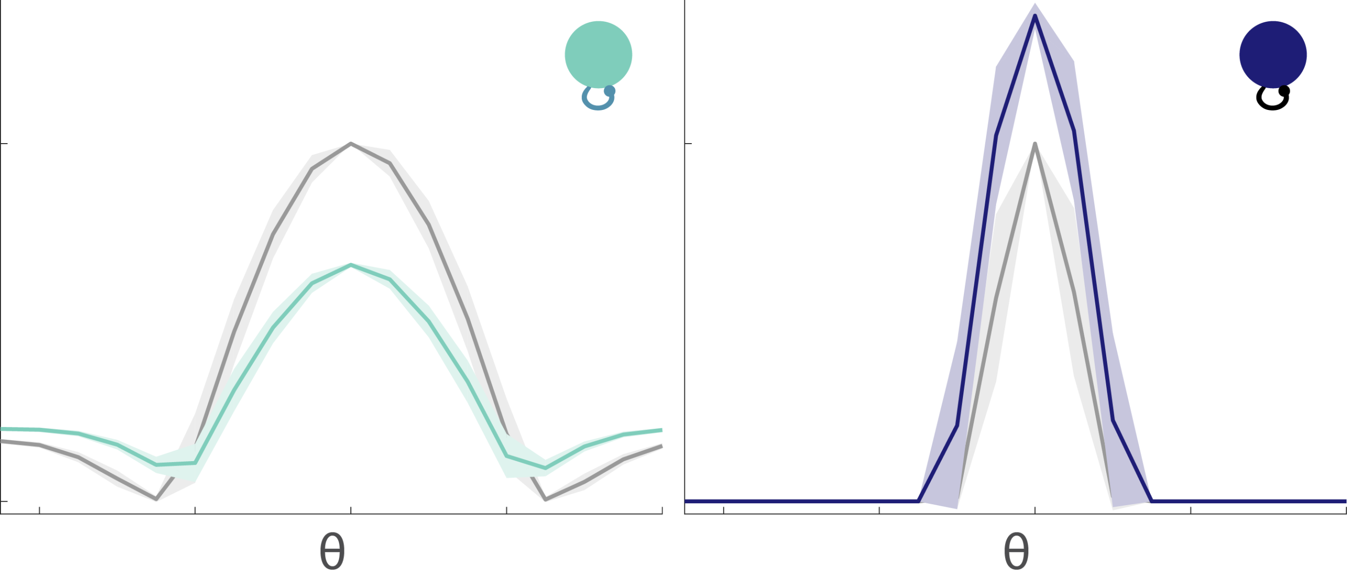
Fig. 9: Tuning curves change after adaptation. Tuning curves for early responses as shown in Fig.8 are in grey. After adaptation, the tuning curves are suppressed for the excitable neurons (left, light green), but facilitated for the mellow neurons (right, dark blue).
We showed that E/I balance works hand-in-hand with adaptation to produce a representation that is both efficient and accurate. Sure, we could’ve allowed adaptation to result in a perceptual bias. Our model doesn’t exclude that possibility, but we paid particular attention to the short-term effects of adaptation, and to the subtle changes that adaptation produces in neuron tuning without degrading the network’s ability to accurately encode the stimulus. The bigger picture here is that variability is part of the optimal solution rather than a problem.
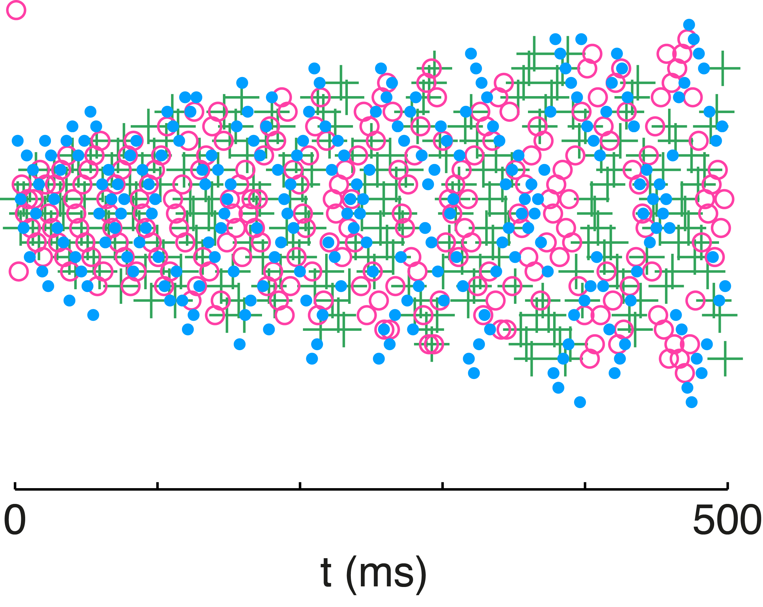
Fig. 10: Variability in network neuron responses. The spike rasters from the network are color coded for each stimulus presentation. The stimulus was identical across trials but preceded by a different randomized stimulus sequence. Individual neuron rasters are organized horizontally so that each line represents the spikes from a given neuron.
We illustrate that principle with the overlaid spike rasters in Figure 10 in which the network is presented with the same stimulus on three separate occasions. The only difference between those presentations are the randomized stimulus sequences presented before each one. The history dependence of spike-frequency adaptation produces highly variable neuron responses to the same stimulus over different trials. Despite that variability in the spike timing and firing rate of individual neurons, the network output is very accurate across those three presentations of the stimulus. Adaptation is the catalyst for the redistribution of spikes, while E/I balance is the means by which spiking activity is redistributed in a manner that will preserve the representation. With adaptation enforcing an efficient encoding and E/I balance maintaining an accurate representation, the network can have its cake and eat it too.
- Barlow, H. B. Reconstructing the visual image in space and time. Nature 279, 189–190 (1979).
- Laughlin, S. A Simple Coding Procedure Enhances a Neurons Information Capacity. Z. Naturforsch., C, Biosci. 36, 910–912 (1981).
- Series, P., Stocker, A. A. & Simoncelli, E. P. Is the Homunculus ‘Aware’ of Sensory Adaptation? Neural Comput 21, 3271–3304 (2009).
- Solomon, S. G. & Kohn, A. Moving Sensory Adaptation beyond Suppressive Effects in Single Neurons. Current Biology 24, R1012–R1022 (2014).
- Boerlin, M., Machens, C. K. & Denève, S. Predictive Coding of Dynamical Variables in Balanced Spiking Networks. PLoS Comput Biol 9, e1003258–16 (2013).

Update: see the full pre-print here https://www.biorxiv.org/content/early/2017/11/03/211748
LikeLike